Deep Learning
Supervised with Nonlinear Models
Supervised learning is
- Predict $y$ from input $x$
- Suppose model/hypothesis is $h_\theta(x)$
Previous methods have considered
- Linear regression : $h_\theta(x) = \theta^Tx$
- Kernel method : $h_\theta(x) = \theta^T \phi(x)$
Both are linear in $\theta$
Now consider models that are nonlinear in both
- Parameters : $\theta$
- Inputs : $x$
The most common of which is the neural network
Cost/Loss Function
Define least-squares cost for one sample $$ J^{(i)}(\theta) = \frac{1}{2} ( h_\theta(x^{(i)}) - y^{(i)})^2 $$ and mean-square cost for the dataset $$ J(\theta) = \frac{1}{n} \sum_{i=1}^{n} J^{(i)}(\theta) $$
Optimisers
SGD or it’s variants is commonly used $$ \theta := \theta - \alpha \nabla_\theta J(\theta) $$ with $\alpha > 0$
Hardware parallelisation means that it’s often faster to compute the gradient of $B$ examples simultaneously
$\Rightarrow$ Mini-batch SGD is most commonly used
Neural Networks
Refers to any type of nonlinear model/parameterisation $h_\theta(x)$ that involves matrix multiplications and other entrywise nonlinear operations
Activation Function
A (1D) nonlinear function that maps $\mathbb{R}$ to $\mathbb{R}$
Common ones include
- ReLU : Rectified Linear Unit
Single Neuron
$$ h_\theta(x) = ReLU(w^Tx + b) $$
- Input : $x \in \mathbb{R}^d$
- Weights : $w \in \mathbb{R}^d$
- Bias : $b \in \mathbb{R}$
Stacking Neurons
Enabels more complex networks
[Example] Two-layer Fully-connected Network
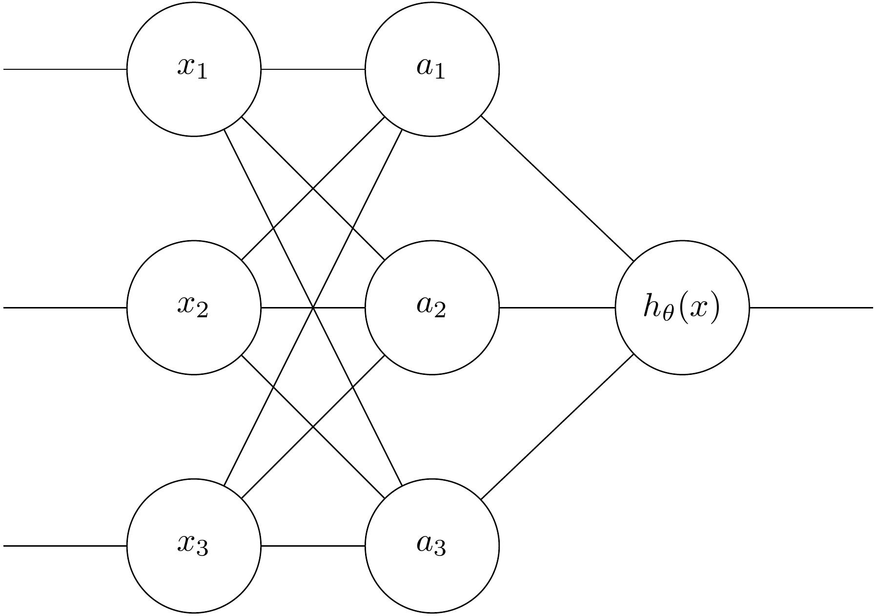
For a hidden layer with three neurons $$ a_1 = ReLU(w_1^T x + b_1) \\ a_2 = ReLU(w_2^T x + b_2) \\ a_3 = ReLU(w_3^T x + b_3) $$ Or equivalently $$ \begin{aligned} &z_i = (w_i^{[1]})^T x + b_i^{[1]} \quad \forall i \in [1,\dots,m] \cr & a_i = ReLU(z_i) \cr & a = [ a_1,\ \dots,\ a_m ]^T \cr & h_\theta(x) = (w^{[2]})^T a + b^{[2]} \end{aligned} $$
Vectorisation
- Simplify expression using more matrix/vector notation
- Important in speeding up neural networks
- Takes advantage of optimised linear algebra packages such as LAPACK/BLAS
- Leverages GPU parallelism
Concatentae weights/inputs/outputs as $$ W^{[i]} = \begin{bmatrix} -\ w^{[i]\top}_1 \ - \cr \vdots \cr -\ w^{[i]\top}_m \ - \end{bmatrix} \in \mathbb{R}^{m\times d} $$ To get $$ \underbrace{ \begin{bmatrix} z^{[i]}_1 \cr \vdots \cr z^{[i]}_m \end{bmatrix} }_{z \in \mathbb{R}^{m\times 1}} = \underbrace{ \begin{bmatrix} -\ w^{[i]\top}_1 \ - \cr \vdots \cr -\ w^{[i]\top}_m \ - \end{bmatrix} }_{W^{[1]} \in \mathbb{R}^{m\times d}} \underbrace{ \begin{bmatrix} x_1 \cr \vdots \cr x_d \end{bmatrix} }_{x \in \mathbb{R}^{d\times 1}} + \underbrace{ \begin{bmatrix} b^{[1]}_1 \cr \vdots \cr b^{[1]}_m \end{bmatrix} }_{b^{[1]} \in \mathbb{R}^{m\times 1}} $$ Or equivalently $$ \begin{aligned} &z = W^{[1]}x + b^{[1]} \cr &a = ReLU(W^{[1]} + b^{[1]}) \cr &h_\theta(x) = W^{[2]} a + b^{[2]} \end{aligned} $$
$\theta$ consists of weights $W^{[i]}$ and biases $b^{[i]}$
Each layer consists of the pair $(W^{[i]}, b^{[i]})$
Multi-Layer Network
- Can stack more layers to get a deeper fully-connected neural network
- If you let $a^{[0]} = x$ and $a^{[r]} = h_\theta(x)$
$$ a^{[k]} = \text{ReLU}\left( W^{[k]} a^{[k-1]} + b^{[k]} \right), \quad \forall k=1,\dots,r-1 $$
Connection to Kernel Method
Deep learning is a method to automatically learn the best feature map (or representation) $$ h_\theta(x) = W^{[r]} \phi_\beta(x) + b^{[r]} $$ With $\beta: a^{[r-1]} = \phi_\beta(x)$ as the feature map
The neural network is therefore a linear regression over the learnt (nonlinear) feature map $\phi_\beta$
Backpropagation
Aka auto-differentiation
Compute the gradient of the loss $\nabla J^{(j)} (\theta)$ efficiently
Theorem (Informally)
Suppose a differentiable circuit of size $N$ computes a real-valued function $f:\mathbb R^l \rightarrow \mathbb R$. The gradient $\nabla f$ can be computed in $O(N)$ time by a circuit of size $O(N)$
Chain Rule
For variables $\theta_1, \dots, \theta_p$ and intermediate variables $g_1, \dots, g_k$ $$ \begin{aligned} g_j = g_j(\theta_1, \dots, \theta_p) \cr J = J(g_1, \dots, g_k) \end{aligned} $$ The chain rule states $$ \frac{\partial J}{\partial \theta_i} = \sum^{k}_{j=1} \frac{\partial J}{\partial g_j} \frac{\partial g_j}{\partial \theta_i} $$