Generative Learning
Generative learning is a different approach to learning as opposed to discriminative learning. It tries to model $p(x|y)$ and $p(y)$ instead of learning $p(y|x)$ directly.
- $p(x|y)$ : Distribution of the target’s features
- $p(y)$ : Class priors
It uses Bayes rule to calculate posterior distribution $p(y|x)$ $$ p(y|x) = \frac{p(x|y) p(y)}{p(x)} $$ And can be simplified when using for prediction because the denominator is constant and doesn’t matter $$ \arg \max_y P(y|x) = \arg \max_y p(x|y) p(y) $$
Multivariate Normal Distribution
The multivariate normal distribution in $d$-dimensions is parameterised by:
- Mean Vector : $\mu \in \mathbb{R}^d$
- Covariance Matrix : $\Sigma \in \mathbb{R}^{d\times d}$
Where $\Sigma$ is symmetric and positive semi-definite (PSD)
The density of $\mathcal{N} (\mu, \Sigma)$ is $$ p(x; \mu, \Sigma) = \frac{1}{(2\pi)^{d/2}|\Sigma|^{1/2}} \exp \left( -\frac{1}{2} (x-\mu)^T \Sigma^{-1} (x-\mu) \right) $$ Where $|\Sigma|$ is the determinant of $\Sigma$
Mean
Is given by $\mu$ $$ \mathbb{E}[X] = \int_x{ x\ p(x; \mu,\Sigma)\ dx } = \mu $$
Covariance
Is defined as $$ Cov(X) = \mathbb{E} \left[ \ (X-\mathbb{E}[X])(X-\mathbb{E}[X])^T \ \right] $$
$$ Cov(X) = \mathbb{E}[XX^T] - (\mathbb{E}[X])(\mathbb{E}[X])^T $$
As covariance increases, the distribution becomes more spread out. Off-diagonal terms skew the distribution.
The standard normal distribution has zero mean and identity covariance.
Gaussian Discriminant Analysis (GDA)
For a classification problem with continuous input features, the GDA model assumes that $p(x|y)$ is distributed according to a multivariate normal distribution $$ \begin{aligned} y &\sim \text{Bernoulli}(\phi) \cr x|y=0 &\sim \mathcal{N}(\mu_0, \Sigma) \cr x|y=1 &\sim \mathcal{N}(\mu_1, \Sigma) \end{aligned} $$ Which expands to $$ \begin{aligned} p(y) &\sim \phi^y (1-\phi)^{1-y} \cr p(x|y=0) &\sim \frac{1}{(2\pi)^{d/2}|\Sigma|^{1/2}} \exp \left( -\frac{1}{2} (x-\mu_0)^T \Sigma^{-1} (x-\mu_0) \right) \cr p(x|y=1) &\sim \frac{1}{(2\pi)^{d/2}|\Sigma|^{1/2}} \exp \left( -\frac{1}{2} (x-\mu_1)^T \Sigma^{-1} (x-\mu_1) \right) \cr \end{aligned} $$ This model usually sets $\Sigma_0 = \Sigma_1 = \Sigma$
The log-likelihood is $$ \begin{aligned} l(\phi, \mu_0, \mu_1, \Sigma) &= log \prod_{i=1}^{n} p(x^{(i)}, y^{(i)}; \phi, \mu_0, \mu_1, \Sigma) \cr &= \log \prod_{i=1}^{n} p(x|y; \mu, \mu, \Sigma)\ p(y;\phi) \end{aligned} $$ And the maximum likelihood estimates of the parameters can be found by maximising $l$ w.r.t the parameters $$ \phi = \frac{1}{n} \sum_{i=1}^{n} 1{ y^{(i)}=1 } $$
$$ \mu_0 = \frac{\sum_{i=1}^n 1{ y^{(i)}=0 } x^{(i)}} {\sum_{i=1}^n 1{ y^{(i)}=0 }} $$
$$ \mu_1 = \frac{\sum_{i=1}^n 1{ y^{(i)}=1 } x^{(i)}} {\sum_{i=1}^n 1{ y^{(i)}=1 }} $$
$$ \Sigma = \frac{1}{n} \sum_{i=1}^{n} (x^{(i)} - \mu_{y^{(i)}}) (x^{(i)} - \mu_{y^{(i)}})^T $$
Graphically, the algorithm is learning the two gaussian distributions
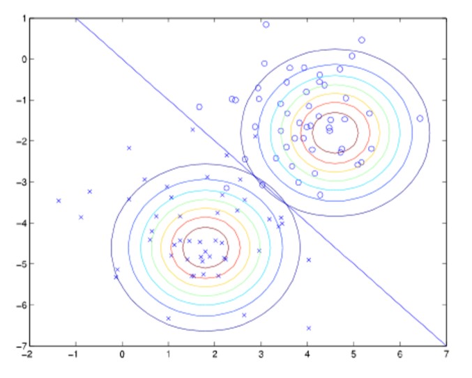
The decision boundary is separating hyperplane between the two distributions
GDA and Logistic Regression
Similarities
Expressing $y$ as a function of $x$ $$ p(y=1|x; \phi, \Sigma, \mu_0, \mu_1) = \frac{1}{1 + \exp(-\theta^Tx)} $$ Has the exact same form as logistic regression
Differences
GDA and logistic regression will generally give different decision boundaries because:
- $p(x|y)$ is Gaussian implies $p(y|x)$ is Logistic
- But $p(y|x)$ is Logistic does not imply that $p(x|y)$ is Gaussian
Conclusion
GDA makes stronger modelling assumptions than logistic regression
- If assumptions are correct, GDA will find better fits
- If $p(x|y)$ is gaussian with shared covariance $\Sigma$, GDA is asymptotically efficient:
As $n \rightarrow \infty$, no algorithm is strictly better than GDA
Comparison
| GDA | Logistic |
|---|---|
| Stronger modelling assumptions | Less sensitive to modelling errors |
| More data efficient | More robust |
[*] In practise logistic regression is used more often than GDA
Naive Bayes
The naive bayes model can be used for classification with discrete-valued input features. (Similar to GDA but with discrete-valued $x$)
Procedure:
Encode set of features into a vocabulary. Dimension of $x$ equals size of vocabulary
But the number of parameters grows with $\large 2^\text{size of vocabulary}$ and quickly becomes too large for an explicit representation
Naive Bayes Assumption
To simplify the model we can make a very strong assumption, the naive bayes assumption:
Assume that the $x$’s are conditially independent given $y$
Example
If an email is spam ($y=1$) and word $x_1$ is apple and word $x_2$ is car
Knowing that $y=1$ and $x_1 = apple$ gives no information about $x_2 = car$ $$ p(x_2 | y) = p(x_2 | y, x_1) $$
[*] This does not say that $x_1$ and $x_2$ are independent
$$ \begin{aligned} p(&x_1, \dots, x_{5000} | y) \cr &= p(x_1|y) p(x_1|y,x_1) \dots p(x_{5000}|y,x_1\dots x_{4999}) \cr \end{aligned} $$ Using the naive bayes assumption the probability can be decomposed into $$ \begin{aligned} p(&x_1, \dots, x_{5000} | y) \vphantom{\prod} \cr &= p(x_1|y) p(x_1|y) \dots p(x_{5000}|y) \vphantom{\prod} \cr &= \prod_{j=1}^d p(x_j | y) \end{aligned} $$ The NB assumption is extremely strong, but the algorithm works well on many real life problems.
Parameterisation
The joint likelihood is $$ \mathcal{L}(\phi_y, \phi_{j|y=0}, \phi_{j|y=1}) = \prod_{i=1}^{n} p(x^{(i)}, y^{(i)}) $$ Maximise w.r.t $\phi_y$, $\phi_{j|y=0}$ and $\phi_{j|y=1}$ $$ \begin{aligned} \phi_{j|y=1} &= \frac{\sum_{i=1}^n 1{ x_k^{(i)}=1 \wedge y^{(i)}=1 }} {\sum_{i=1}^n 1{ y^{(i)}=1 }} \cr \phi_{j|y=0} &= \frac{\sum_{i=1}^n 1{ x_k^{(i)}=1 \wedge y^{(i)}=0 }} {\sum_{i=1}^n 1{ y^{(i)}=0 }} \cr \phi_{y} &= \frac{\sum_{i=1}^n 1{ y^{(i)}=1 }}{n} \end{aligned} $$ To make a prediction, find the highest possiblity from $$ p(y=1|x) = \frac{p(x|y=1) p(y=1)}{p(x)} $$
Laplace Smoothing
- The first time the Naive Bayes algorithm encounters a new feature, it cannot estimate the probability
$$ \begin{aligned} p(y=1|x) &= \frac { \prod_{j=1}^{d} p(x_j|y=1) p(y=1) } { \prod_{j=1}^{d} p(x_j|y=1) p(y=1) + \prod_{j=1}^{d} p(x_j|y=0) p(y=0) } \cr p(y=1|x) &= \frac{0}{0} \end{aligned} $$
- Because $\prod p(x_j|y)$ includes $p(x_{new}|y)$ which is $0$ and therefore it always obtains $0/0$.
- It is a bad idea to estimate a previously unseen event to zero.
Solution
Introduce Laplace smoothing $$ \phi_j = \frac{1 + \sum_{i=1}^{n} 1 { z^{(i)}=j }} {k+n} $$
- Add $1$ to the numerator
- Add $k$ to the denominator
- $\sum_{j=1}^{k} \phi_j=1$ still holds
- $\phi_j \neq 0$ for all $j$
Under certain (strong) conditions
- Laplace smoothing gives the optimal estimator