Regularization
There is a tradeoff between bias (underfitting) and variance (overfitting). The optimal tradeoff requires computing the correct model complexity.
Model Complexity : Can be a function of the parameters ($l_2$ norm) and not just the number of parameters
Regularization : Allows us to:
- Control model complexity
- Prevent overfitting
Regularizer Function
A regularizer $R(\theta)$, is a function which measures model complexity. It is usually nonnegative.
In classical methods : $R(\theta)$ depends only on parameters $\theta$
In modern methods : $R(\theta,x,y)$ can depend on the data
$R(\theta)$ is added to the training loss/cost to get the regularized loss $J_\lambda$ $$ J_\lambda(\theta) = \underbrace{J(\theta)}_\text{training loss} + \lambda \underbrace{R(\theta)}_\text{regularizer} $$ Parameter $\lambda$ : Determines the balance between training loss and regularization. A small $\lambda$ serves as a “tiebreaker” for equally effective models.
Weight Decay
One of the most commonly used is $l_2$ regularization. In deep learning it is also known as weight decay, where parameter weights gradually grow smaller over time.
The update rule for weight decay is $$ \theta \quad \leftarrow \underbrace{(1 - \lambda \eta)\ \cdot }_\text{decaying weights} \theta - \eta \nabla J(\theta) $$ Is equivalent to $l_2$ regularization $$ \theta \leftarrow \theta - \eta( \underbrace{\nabla J(\theta)}_\text{loss} \quad + \underbrace{\lambda \theta}_\text{regularizer} ) $$
Imposing Inductive Bias / Structure
Regularization can also impose inductive bias or structure.
It imposes structure that narrows the search space. This reduces the complexity of the model family and improves generalization
BUT, if the structure is wrong it will increase bias / underfitting.
Implicit Regularization Effect
Implicit regularization of optimizers / implicit bias / algorithmic regularization is the concept that “optimizers can implicitly impose structure” on models.
It is a new phenomenon observed in deep learning which might be responsible for performance in the overparameterized regime.
Background
In classical machine learning, loss functions have a unique global minima that all optimizers converge to. However in deep learning, the loss often has multiple approximate global minima.
Different optimizers tend to converge to different types of global minima. The different minima have different properties that make some generalize better than others.
Example
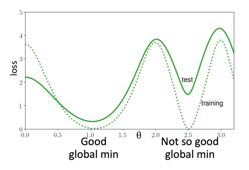
Illustration of how certain minimas generalize better
Components which provide Regularization
Open research question, but empirically:
- Larger initial learning rates
- Smaller initialization
- Smaller batch size
- Momentum
Types of Global Minima which Generalize well
A conjecture is that stochasticity in the optimizer helps to find flatter minima, which generalize better
Cross Validation
Cross validation is a method of training and testing models on different portions of data to access the performance (true generalization) of the model.
Simple (Hold-Out) Cross Validation
- Split dataset $S$ into $S_\text{train}$ (approx. 70%) and $S_\text{test}$(approx. 30%)
- Train various models on $S_\text{train}$ and test on $S_\text{test}$
- Pick model with the smallest error
This methods generates better estimates of a model’s generalization / test error, because it is tested on unseen data.
Disadvantages
It “wastes” around 30% of the dataset, even if the model is subsequently retrained on the entire dataset.
K-Fold Cross Validation
- Split the data into $k$ disjoint subsets
- Test each model on all but one of the subsets
- Select model with the smallest error
- Retrain model on entire dataset
Is a method to reduce the amount of data wasted. It only holds out $\frac{1}{k}$ of the data.
Advantages : More efficient at using data, it uses $\frac{k-1}{k}$ of the data
Disadvantage : Computationally expensive, each model is trained $k$ times
$k=10$ is a common choice
Leave-one-out Cross Validation
Is a more extreme variant where $k = m$, the number of training examples. At every iteration, only one training example is left out.
Bayesian Regularization
| Frequentist | Bayesian |
|---|---|
| $\theta$ unknown constant-valued | $\theta$ is a random variable |
| Maximum likelihood estimation (MLE) | Maximum a posterior (MAP) |
| $\arg \max_\theta \prod p(y | x;\theta)$ | $\arg \max_\theta \prod p(y | x;\theta) \ p(\theta)$ |
Previous sections treated the parameter fitting as a maximum likelihood estimation (MLE) problem. The parameters $\theta$ are treated as an unknown constant-value. $$ \theta_\text{MLE} = \arg \max_\theta \prod^n_{i=1} {p(y^{(i)}\ | x^{(i)} ;\ \theta)} $$ An alternative interpretation is the Bayesian view, where $\theta$ is a random variable (RV).
Bayesian Prediction
In “fully Bayesian” prediction, the prediction is the average w.r.t. the posterior $p(\theta | S)$ over $\theta$ $$ \mathbb E [y | x, S] = \int_y y\ p(y|x,S)\ dy $$ Where the posterior distribution on the class label is $$ p(y|x,S) = \int_\theta p(y|x,\theta) \ p(\theta|S) \ d\theta $$ And the posterior distribution on the class labels is computed from Bayes rule $$ p(\theta | S) = \frac {\left( \prod p(y|x,\theta) \right) p(\theta)} {\int_\theta \left( \prod p(y|x,\theta) \right) p(\theta) \ d\theta} $$
Maximum A Posteriori Approximation
In general it is very difficult / expensive to compute the posterior distribution. There is no closed-form solution, and the high-dimension $\theta$ makes it intractable.
A common approximation is to use a single point estimate, the maximum a posteriori (MAP) estimate $$ \theta_\text{MAP} = \arg \max_\theta \prod^n_{i=1} {p(y^{(i)}\ | x^{(i)} ;\ \theta)} \ p(\theta) $$
Choice of Prior $p(\theta)$
A common choice is $$ \theta \sim \mathcal{N} (0, \tau^2 I) $$ Which has a smaller norm than MLE. This reduces the chance of overfitting.